CVXGEN: Code Generation for Convex Optimization

Example: Model Predictive Control (MPC)

This example, from control systems, shows a typical model predictive control problem. See the paper by Mattingley, Wang and Boyd for some detailed examples of MPC with CVXGEN.

Optimization problem

We will model the optimization problem

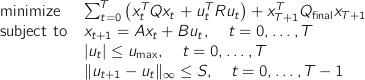
$begin{array}{ll} mbox{minimize} & sum_{t=0}^T left( x_t^T Q x_t + u_t^T R u_t right) + x_{T+1}^T Q_mathrm{final} x_{T+1} mbox{subject to} & x_{t+1} = Ax_t + Bu_t, quad t=0,ldots,T & |u_t| leq u_mathrm{max}, quad t=0,ldots,T & |u_{t+1} - u_t|_infty leq S, quad t=0,ldots,T-1 end{array}$

with optimization variables

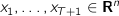$x_1, ldots, x_{T+1} in mathbf{R}^n$ (state variables)
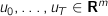$u_0, ldots, u_{T} in mathbf{R}^m$ (input variables)

and parameters

$A in mathbf{R}^{ntimes n}$ (dynamics matrix)
$B in mathbf{R}^{ntimes m}$ (transfer matrix)
$Q in mathbf{S}^{ntimes n}_+$ (state cost)
$Q_mathrm{final} in mathbf{S}^{ntimes n}_+$ (final state cost)
$R in mathbf{S}^{m times m}_+$ (input cost)
$x_0 in mathbf{R}^n$ (initial state)
$u_mathrm{max} in mathbf{R}_+$ (amplitude limit)
$S in mathbf{R}_+$ (slew rate limit)

CVXGEN code

dimensions
  m = 2  # inputs.
  n = 5  # states.
  T = 10  # horizon.
end

parameters
  A (n,n)  # dynamics matrix.
  B (n,m)  # transfer matrix.
  Q (n,n) psd  # state cost.
  Q_final (n,n) psd  # final state cost.
  R (m,m) psd  # input cost.
  x[0] (n)  # initial state.
  u_max nonnegative  # amplitude limit.
  S nonnegative  # slew rate limit.
end

variables
  x[t] (n), t=1..T+1  # state.
  u[t] (m), t=0..T  # input.
end

minimize
  sum[t=0..T](quad(x[t], Q) + quad(u[t], R)) + quad(x[T+1], Q_final)
subject to
  x[t+1] == A*x[t] + B*u[t], t=0..T  # dynamics constraints.
  abs(u[t]) <= u_max, t=0..T  # maximum input box constraint.
  norminf(u[t+1] - u[t]) <= S, t=0..T-1  # slew rate constraint.
end